The MNIST dataset is a set of 70,000 human-labeled 28 x 28 greyscale images of individual handwritten digits. It is a subset of a larger dataset available from NIST - The National Institute of Standards and Technology. In this tutorial, you'll create your own handwritten digit recognizer using a multilayer neural network trained on the MNIST dataset.
- PHP 8.3 or above
- Tensor extension 4.0+ for faster training and inference
- GD extension
Clone the project locally using Composer:
$ composer create-project rubix/mnistNote: Installation may take longer than usual due to the large dataset.
Then, install the Tensor Ext 4.x and GD extensions if they have not been installed yet. You can install the Tensor Ext extension using PIE like in the example below:
pie install rubix/tensor_ext:^4.1In this tutorial, we'll use Rubix ML to train a deep learning model called a Multilayer Perceptron to recognize the numbers in handwritten digits. For this problem, a classifier will need to be able to learn lines, edges, corners, and a combinations thereof in order to distinguish the numbers in the images. In the figure below, we see a snapshot of the features at one layer of a neural network trained on the MNIST dataset. The illustration shows that at each layer, the network builds a more detailed depiction of the training data until the digits are distinguishable by a Softmax layer at the output.
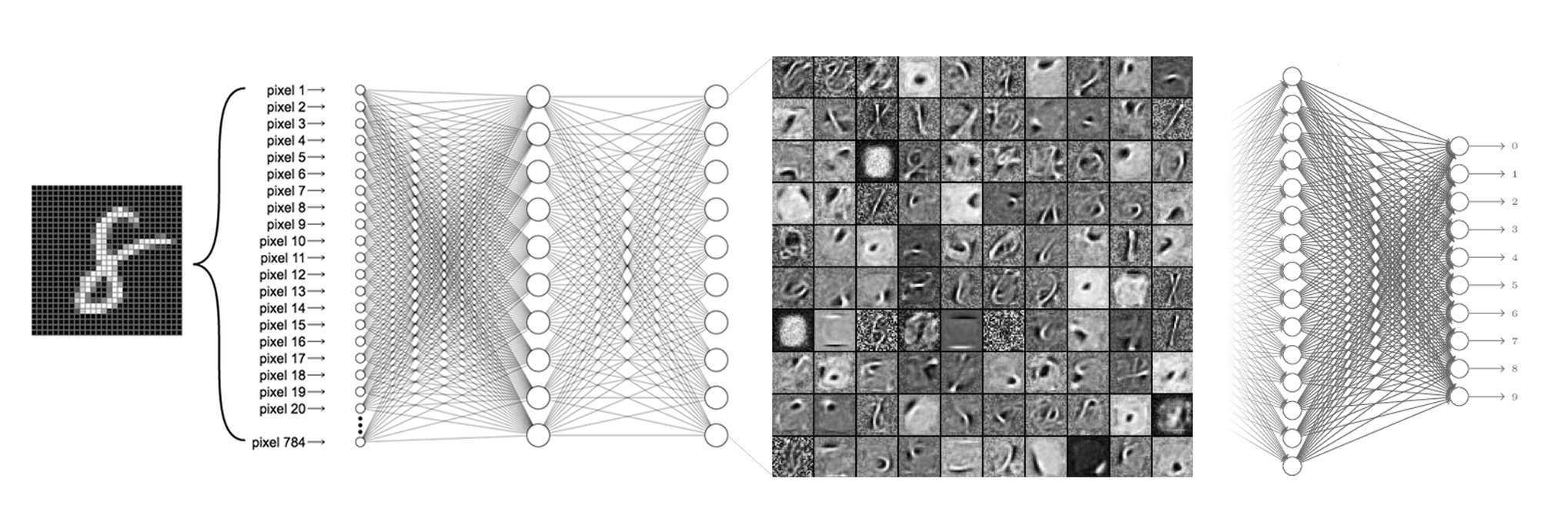
Note: The source code for this example can be found in the train.php file in project root.
The MNIST dataset comes to us in the form of 60,000 training and 10,000 testing images organized into subfolders where the folder name is the human-annotated label given to the sample. We'll use the imagecreatefrompng() function from the GD library to load the images into our script and assign them a label based on the subfolder they are in.
Since we need both splits, we'll extract them in one pass over the two directory names, instantiating a separate Labeled dataset object from the samples and labels of each.
use Rubix\ML\Datasets\Labeled;

$datasets = [];

foreach (['training', 'testing'] as $dir) {
    $samples = $labels = [];

    for ($label = 0; $label < 10; $label++) {
        foreach (glob("$dir/$label/*.png") as $file) {
            $samples[] = [imagecreatefrompng($file)];
            $labels[] = "#$label";
        }
    }

    $datasets[] = new Labeled($samples, $labels);
}

[$training, $testing] = $datasets;
From this point on, $training holds the 60,000 images that the network will learn from, and $testing holds the 10,000 that it will be scored against. Note that none of the testing samples will ever be used to fit a transformer or update a weight - $testing is reserved as the validation set that scores the model at the end of every epoch.
We're going to use a transformer Pipeline to shape the dataset into the correct format for our learner. We know that the size of each sample image in the MNIST dataset is 28 x 28 pixels, but just to make sure that future samples are always the correct input size we'll add an Image Resizer. Then, to convert the image into raw pixel data we'll use the Image Vectorizer which extracts continuous raw color channel values from the image. Since the sample images are black and white, we only need to use 1 color channel per pixel. Rubix ML 3.0 uses a high-level type system where features are typed as either categorical or continuous, so we'll run the vectorized output through the Float Type Converter to make sure the pixel values are interpreted as continuous float features. At the end of the pipeline we'll center and scale the dataset using the Z Scale Standardizer to help speed up the convergence of the neural network.
Unlike the other three, the standardizer is stateful - it learns the mean and standard deviation of every pixel column from the data it is fitted on. That means inference has to reuse those exact numbers or the network will receive inputs on a completely different scale than it was trained on. To make that possible, we'll wrap the pipeline in a Persistent Transformer meta-estimator, which is to transformers what Persistent Model is to learners. It adds save() and load() methods that delegate to the base object, and it needs a Persister object to tell it where to store its state. Just like before, we'll use the Filesystem persister with history mode enabled.
use Rubix\ML\Transformers\PersistentTransformer;
use Rubix\ML\Transformers\Pipeline;
use Rubix\ML\Transformers\ImageResizer;
use Rubix\ML\Transformers\ImageVectorizer;
use Rubix\ML\Transformers\FloatTypeConverter;
use Rubix\ML\Transformers\ZScaleStandardizer;
use Rubix\ML\Persisters\Filesystem;

$transformer = new PersistentTransformer(
    base: new Pipeline([
        new ImageResizer(28, 28),
        new ImageVectorizer(grayscale: true),
        new FloatTypeConverter(),
        new ZScaleStandardizer(),
    ]),
    persister: new Filesystem('transformer.rbx', true)
);
Before we can transform anything, the transformer has to be fitted. We'll fit it on the training set alone - fitting on both would leak the mean and standard deviation of the testing pixels into training and give us an optimistic picture of how the model generalizes. The fit() method delegates to the pipeline, which works on a clone of the dataset and leaves the original samples untouched, so this call only learns the standardizer's statistics and does not transform anything yet.
$transformer->fit($training);Now, we'll go ahead and instantiate our Multilayer Perceptron classifier. Let's consider a neural network architecture suited for the MNIST problem consisting of 4 groups of Dense neuronal layers of 256 neurons each, each followed by a GELU activation layer and a mild Dropout layer set to 0.1 to act as a regularizer. GELU is a smooth, non-monotonic activation function that has been shown to train faster and generalize better than the classic ReLU. The third group disables the bias term of its Dense layer and is followed by a Batch Norm layer which normalizes the activations of the previous layer such that the mean activation is close to 0 and the standard deviation is close to 1. Batch Norm reduces the amount of covariate shift within the network, which makes it possible to converge faster under some circumstances. The output layer adds an additional layer of neurons with a Softmax activation making this particular network architecture 6 layers deep.
Next, we'll set the batch size to 32. The batch size is the number of samples sent through the network at a time. A smaller batch keeps memory usage in check but introduces more noise into each gradient estimate. To compensate, we'll set the gradient accumulation steps to 4, which waits until the gradients across 4 batches have been accumulated before applying a single update - giving us an effective batch size of 128 while only ever keeping 32 samples in memory at once.
We'll also specify an optimizer and a learning rate scheduler which determines the update step of the Gradient Descent algorithm. The Adam optimizer uses a combination of Momentum and RMS Prop to make its updates and usually converges faster than standard stochastic Gradient Descent. In Rubix ML 3.0 the optimizer takes a Scheduler object which dictates the learning rate over the course of training. We'll use the simple Constant scheduler which holds the learning rate at 0.0001 for the duration of the training run. To keep the updates numerically stable we'll cap the magnitude of the gradients by setting the maximum gradient norm to 1.0.
Finally, we'll tell the learner to train for a maximum of 100 epochs, and to score the model on the validation dataset every single epoch (evalInterval: 1). There are two independent early stopping criteria. The first is window: 5 - if the validation score fails to improve on any of 5 consecutive evaluations, training halts. The second is minChange: 1e-5 - if the epoch's average loss moves by less than this from the previous epoch, the run has converged and training halts too. Both keep the run from overfitting by effectively unlearning some of the noise in the dataset.
use Rubix\ML\Loggers\Screen;
use Rubix\ML\PersistentModel;
use Rubix\ML\Classifiers\MultilayerPerceptron;
use Rubix\ML\NeuralNet\Layers\Dense;
use Rubix\ML\NeuralNet\Layers\Dropout;
use Rubix\ML\NeuralNet\Layers\Activation;
use Rubix\ML\NeuralNet\Layers\BatchNorm;
use Rubix\ML\NeuralNet\ActivationFunctions\GELU;
use Rubix\ML\NeuralNet\Optimizers\Schedulers\Constant;
use Rubix\ML\NeuralNet\Optimizers\Adam;
use Rubix\ML\Persisters\Filesystem;

$logger = new Screen();

$estimator = new PersistentModel(
    base: new MultilayerPerceptron(
        hiddenLayers: [
            new Dense(256),
            new Activation(new GELU()),
            new Dropout(0.1),
            new Dense(256),
            new Activation(new GELU()),
            new Dropout(0.1),
            new Dense(256, bias: false),
            new BatchNorm(),
            new Activation(new GELU()),
            new Dropout(0.1),
            new Dense(256),
            new Activation(new GELU()),
            new Dropout(0.1),
            new Dense(10),
        ],
        batchSize: 32,
        gradientAccumulationSteps: 4,
        optimizer: new Adam(new Constant(0.0001)),
        maxGradientNorm: 1.0,
        epochs: 100,
        minChange: 1e-5,
        evalInterval: 1,
        window: 5,
    ),
    persister: new Filesystem('model.rbx', true)
);

$estimator->setLogger($logger);
To allow us to save and load the model from storage, we'll wrap the network in a Persistent Model meta-estimator. Persistent Model provides additional save() and load() methods on top of the base estimator's methods. It needs a Persister object to tell it where the model is to be stored. For our purposes, we'll use the Filesystem persister which takes a path to the model file on disk. Setting history mode to true means that the persister will rename the previous file to model.rbx-<timestamp>.old each time we save, keeping track of every past save.
Note that the pipeline lives outside of the Persistent Model. Only the Multilayer Perceptron is persisted as model.rbx, and the preprocessing is persisted alongside it as transformer.rbx by the Persistent Transformer. Keeping the two separate is what lets us swap the preprocessing out later without invalidating a trained network.
Now that the transformer is fitted, we can use it to preprocess both datasets. The apply() method hands the samples to the transformer and modifies them in place, so the 784 raw pixel values of each image become 784 standardized float features. Labels are never touched, and the same dataset object is returned, so the calls chain.
$logger->info('Preprocessing dataset');

$training->apply($transformer);
$testing->apply($transformer);
Next we tell the learner where its validation set lives. In Rubix ML 3.0 the holdOut hyper-parameter was removed and learners no longer carve out a slice of the training data on their own. Instead, setValidationDataset() takes the dataset that will be scored at the end of each evaluation interval, which must be called before train() begins the epoch loop.
$estimator->setValidationDataset($testing);This is what lets us use all 60,000 training images to actually train the network. If we skip this step the learner will still fit every sample, but it has nothing to score against, so progress monitoring, snapshotting, and early stopping are all disabled - it even logs a notice saying as much.
Finally, to start training the neural network, call the train() method on the Estimator instance with the training set as an argument.
$estimator->train($training);We can visualize the training progress at each stage by dumping the values of the loss function and validation metric after training. The progress() method will output an iterator that yields one row per epoch containing the epoch number, the value of the default Multiclass Cross Entropy cost function, the gradient norm, and the score of the F Beta metric. If you'd prefer to work with the validation metric on its own, the scores() method will return a flat array of just the F Beta scores from the last training session.
Note: You can change the cost function and validation metric by setting them as hyper-parameters of the learner.
use Rubix\ML\Extractors\CSV;

$extractor = new CSV('progress.csv', true);

$extractor->export($estimator->progress(), overwrite: true);
The true passed to the constructor enables the header row. Note the overwrite: true on export() - in Rubix ML 3.0 extractors append by default, so without it every run would stack its epochs underneath the previous run's and the resulting chart would be meaningless.
Then, we can plot the values using our favorite plotting software such as Tableu or Excel. If all goes well, the value of the loss should go down as the value of the validation score goes up. Because the validation set is the untouched MNIST testing split, these scores reflect genuine held-out performance rather than performance on data the network was also trained on. Due to snapshotting, the epoch at which the validation score is highest and the loss is lowest is the point at which the values of the network parameters are taken for the final model. This prevents the network from overfitting the training data by effectively unlearning some of the noise in the dataset.
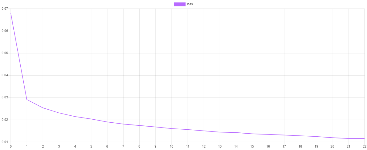
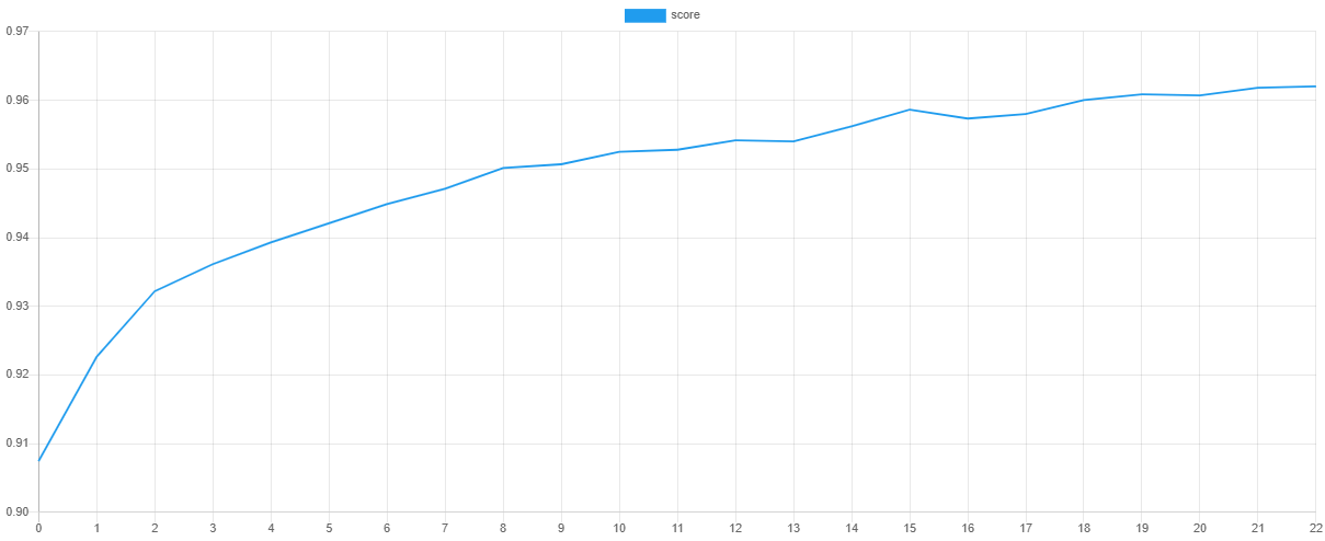
We can save the trained network by calling the save() method provided by the Persistent Model wrapper. The model will be serialized using the RBX serializer, a compact binary format that is the default choice in Rubix ML 3.0. Alternatives like Native PHP serialization also exist if you prefer a more human-readable or language-agnostic encoding.
The transformer gets saved the same way through the Persistent Transformer wrapper. Both objects are needed to make a prediction later - the weights in model.rbx are meaningless without the exact Z Scale Standardizer statistics in transformer.rbx that they were trained against.
$transformer->save();
$estimator->save();
Since training a network on the full MNIST dataset can take hours, we don't want to commit a model to disk on every run. Instead, the script will ask you interactively whether you'd like to keep the model before it saves, defaulting to no.
Now we're ready to execute the training script from the command line.
Cross Validation is a technique for assessing how well the Estimator can generalize its training to an independent dataset. The goal is to identify problems such as underfitting, overfitting, or selection bias that would cause the model to perform poorly on new unseen data.
Fortunately, the MNIST dataset includes an extra 10,000 labeled images that we can use to test the model. Since we haven't used any of these samples to update the network's weights with, we can use them to test the generalization performance of the model. These are the same 10,000 images that were handed to the learner as its validation dataset during training, so the report below is a true out-of-sample measurement. To start, we'll extract the testing samples and labels from the testing folder into a Labeled dataset object.
use Rubix\ML\Datasets\Labeled;

$samples = $labels = [];

for ($label = 0; $label < 10; $label++) {
    foreach (glob("testing/$label/*.png") as $file) {
        $samples[] = [imagecreatefrompng($file)];
        $labels[] = "#$label";
    }
}

$dataset = new Labeled($samples, $labels);In our training script we made sure to save the model before we exited. In our validation script, we'll load the trained model from storage and use it to make predictions on the testing set. Both artifacts have a static load() method that takes a Persister object pointing to the object in storage as its only argument and returns the loaded instance.
Once the model is loaded, we'll call cleanup() on it. After training, the optimizer keeps around a set of internal state buffers (momentum and norm estimates) used to make its updates. Since we're only doing inference now and will never update the weights again, we can ask the optimizer to flush those buffers and release the memory they occupy. cleanup() isn't defined on the Persistent Model itself - it is forwarded to the wrapped Multilayer Perceptron, which is where the optimizer lives.
use Rubix\ML\Transformers\PersistentTransformer;
use Rubix\ML\PersistentModel;
use Rubix\ML\Persisters\Filesystem;

$transformer = PersistentTransformer::load(new Filesystem('transformer.rbx'));

$estimator = PersistentModel::load(new Filesystem('model.rbx'));

$estimator->cleanup();The loaded model only accepts standardized float features, so we have to put the raw images through the same pipeline they went through during training. Because the transformer was loaded with its fitted state intact, calling apply() on the dataset skips the fitting step entirely and goes straight to the transformation.
$logger->info('Preprocessing dataset');

$dataset->apply($transformer);Now we can use the estimator to make predictions on the testing set. The predict() method takes a dataset as input and returns an array of predictions.
$predictions = $estimator->predict($dataset);The cross validation report we'll generate is actually a combination of two reports - Multiclass Breakdown and Confusion Matrix. We'll wrap each report in an Aggregate Report to generate both reports at once under their own key.
use Rubix\ML\CrossValidation\Reports\AggregateReport;
use Rubix\ML\CrossValidation\Reports\ConfusionMatrix;
use Rubix\ML\CrossValidation\Reports\MulticlassBreakdown;

$report = new AggregateReport([
    'breakdown' => new MulticlassBreakdown(),
    'matrix' => new ConfusionMatrix(),
]);
To generate the report, pass in the predictions along with the labels from the testing set to the generate() method on the report. We can print the report to the terminal and then encode the results as JSON and save them to report.json for later inspection.
$results = $report->generate($predictions, $dataset->labels());

echo $results;

$results->toJSON()->saveTo(new Filesystem('report.json'));
Now we're ready to run the validation script from the command line.
$ php validate.phpBelow is an excerpt from an example report. As you can see, our model was able to achieve 99.6% accuracy on the testing set.
{
    "breakdown": {
        "overall": {
            "accuracy": 0.9955000000000002,
            "balanced accuracy": 0.9873923361403957,
            "f1 score": 0.9773124462117178,
            "precision": 0.9773905650775483,
            "recall": 0.9772836696129319,
            "specificity": 0.9975010026678597,
            "negative predictive value": 0.9975024960911097,
            "false discovery rate": 0.02260943492245161,
            "miss rate": 0.02271633038706815,
            "fall out": 0.00249899733214054,
            "false omission rate": 0.0024975039088902307,
            "mcc": 0.9748290851449231,
            "informedness": 0.9747846722807914,
            "markedness": 0.9748930611686581,
            "true positives": 9775,
            "true negatives": 89775,
            "false positives": 225,
            "false negatives": 225,
            "cardinality": 10000
        },
        "classes": {
            "#0": {
                "accuracy": 0.997,
                "balanced accuracy": 0.9937893117335626,
                "f1 score": 0.9847715736040609,
                "precision": 0.9797979797979798,
                "recall": 0.9897959183673469,
                "specificity": 0.9977827050997783,
                "negative predictive value": 0.9988901220865705,
                "false discovery rate": 0.02020202020202022,
                "miss rate": 0.010204081632653073,
                "fall out": 0.0022172949002217113,
                "false omission rate": 0.0011098779134295356,
                "informedness": 0.9875786234671251,
                "markedness": 0.9786881018845501,
                "mcc": 0.9831233129484814,
                "true positives": 970,
                "true negatives": 9000,
                "false positives": 20,
                "false negatives": 10,
                "cardinality": 980,
                "proportion": 0.098
            },
            "#5": {
                "accuracy": 0.9955,
                "balanced accuracy": 0.9833716872369631,
                "f1 score": 0.9746192893401014,
                "precision": 0.9807037457434733,
                "recall": 0.968609865470852,
                "specificity": 0.9981335090030742,
                "negative predictive value": 0.9969294878824433,
                "false discovery rate": 0.0192962542565267,
                "miss rate": 0.03139013452914796,
                "fall out": 0.001866490996925818,
                "false omission rate": 0.003070512117556712,
                "informedness": 0.9667433744739262,
                "markedness": 0.9776332336259166,
                "mcc": 0.9721730562370955,
                "true positives": 864,
                "true negatives": 9091,
                "false positives": 17,
                "false negatives": 28,
                "cardinality": 892,
                "proportion": 0.0892
            }
        }
    },
    "matrix": {
        "#0": {
            "#0": 970,
            "#3": 0,
            "#8": 1,
            "#7": 1,
            "#6": 6,
            "#2": 7,
            "#1": 0,
            "#5": 2,
            "#4": 1,
            "#9": 2
        },
        "#5": {
            "#0": 0,
            "#3": 5,
            "#8": 2,
            "#7": 1,
            "#6": 4,
            "#2": 0,
            "#1": 1,
            "#5": 864,
            "#4": 0,
            "#9": 4
        }
    }
}Congratulations on completing the MNIST tutorial on handwritten digit recognition in Rubix ML. We highly recommend browsing the documentation to get a better feel for what the neural network subsystem can do. What other problems would deep learning be suitable for?
Yann LeCun, Professor The Courant Institute of Mathematical Sciences New York University Email: yann 'at' cs.nyu.edu
Corinna Cortes, Research Scientist Google Labs, New York Email: corinna 'at' google.com
- Y. LeCun et al. (1998). Gradient-based learning applied to document recognition.
The code is licensed MIT and the tutorial is licensed CC BY-NC 4.0.